How does prompt caching work?
Nearly all inference libraries can do it for you. But what's really going on under the hood?
This is episode 3 of a series of shorter blog posts answering questions I received during the course of my work. They discuss common misconceptions and doubts about various generative AI technologies. You can find the whole series here: Practical Questions.
In the previous post we saw what is prompt caching, what parts of the prompts is useful to cache, and explained at a high level why it's so effective. In this post I want to go one step further and explain how in practice inference engines cache prompt prefixes. How can you take a complex system like an LLM, cache some of its computations mid-prompt, and reload them?
Let's find out.
Disclaimer: to avoid overly complex and specific diagrams, the size of the vector and matrices shown is not accurate neither in size nor in shape. Check the links at the bottom of the post for more detailed resources with more accurate diagrams.
LLMs are autoregressive
Large Language Models are built on the Transformer architecture: a neural network design that excels at processing sequence data. Explaining the whole structure of a Transformer goes beyond the scope of this small post: if you're interested in the details, head to this amazing writeup by Jay Alammar about Transformers, or this one about GPT-2 if you're familiar with Transformers but you want to learn more about the decoder-only architecture (which includes all current LLMs).
The point that interests us is that according to the original implementation, during inference the LLM generate text one token at a time in an autoregressive fashion, meaning each new token is predicted based on all previously generated tokens. After producing (or "decoding") a token, that token is appended to the input sequence and the model computes everything all over again to generate the next one. This loop continues until a stopping condition is reached (such as an end-of-sequence token or a length limit).
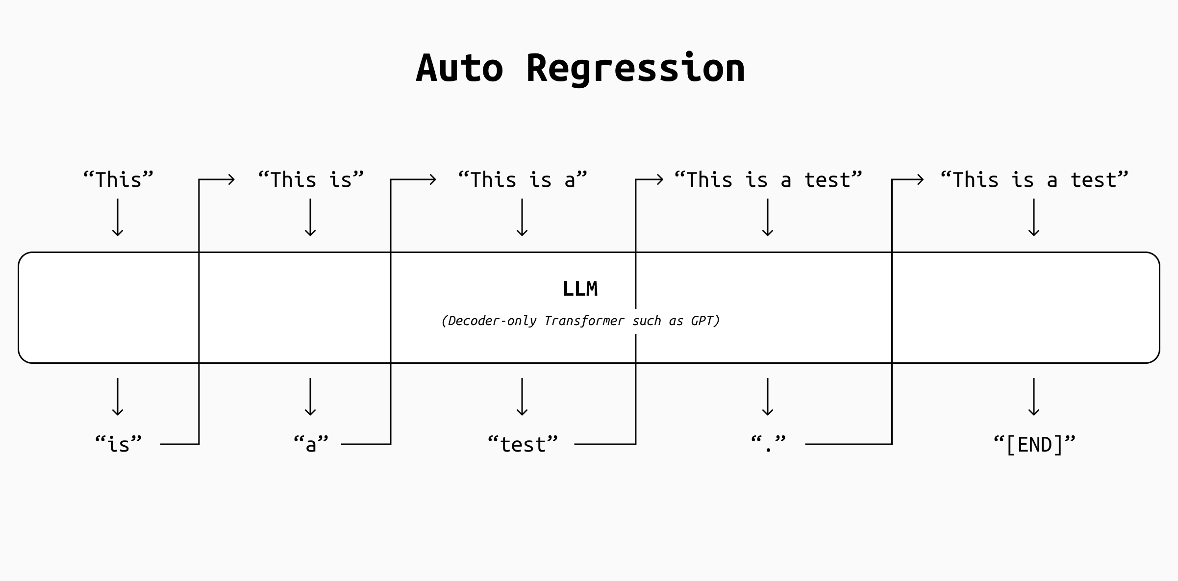
In an autoregressive system, the output is generated token by token by appending the previous pass' output to its input and recomputing everything again. Starting from the token "This", the LLM produces "is" as output. Then the output is concatenated to the input in the string "This is", which is fed again to the LLM to produce "a", and so on until an [END] token is generated. That halts the loop.
This iterative process is very computationally expensive (quadratic time complexity in the number of tokens, so O(n^2) where n is the number of tokens), and the impact is felt especially for long sequences, because each step must account for an ever-growing history of generated tokens.
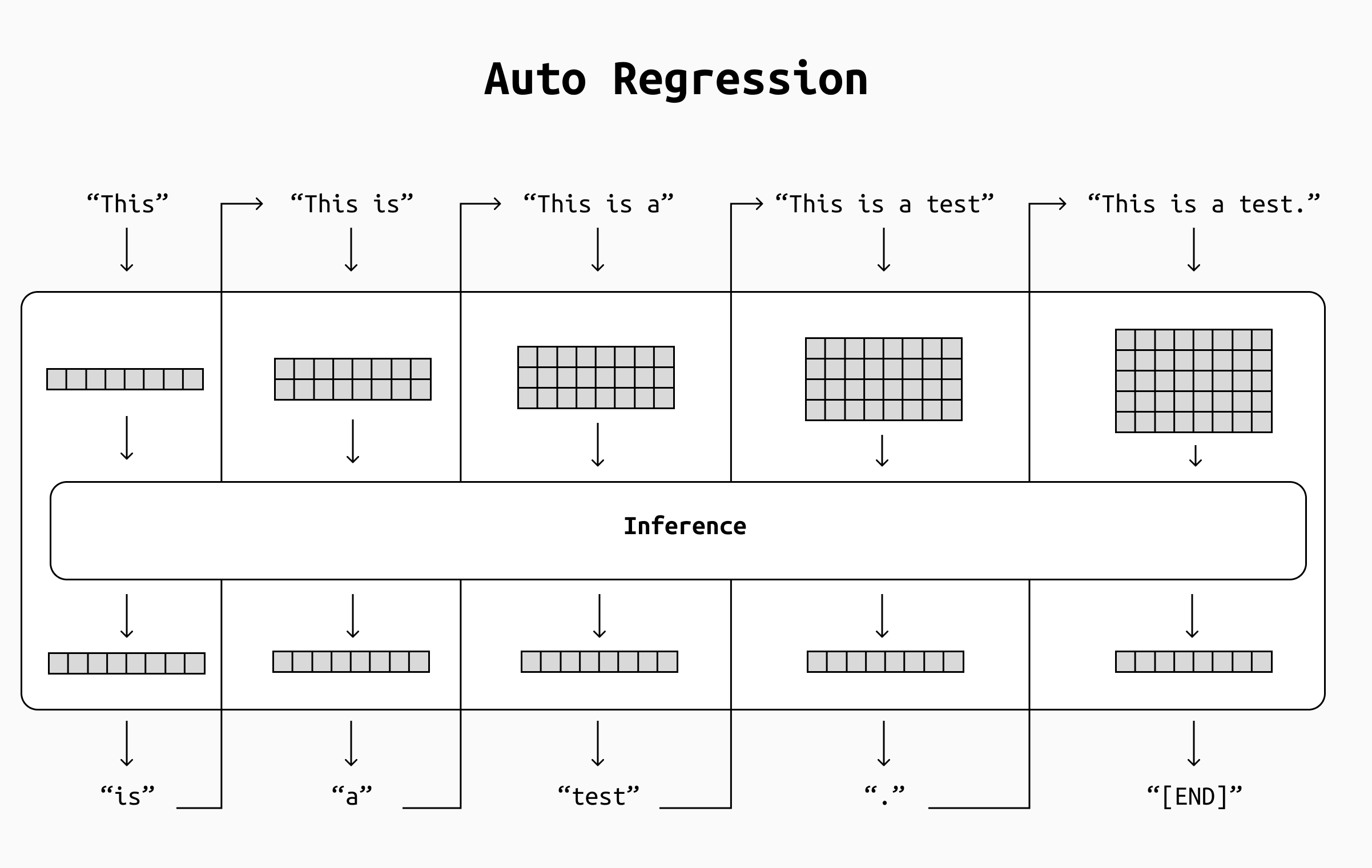
Simplified view of the increasing computation load. At each pass, the increasing length of the input sentence translated into larger matrices to be handled during inference, where each row corresponds to one input token. This means more computations and, in turn, slower inference.
However, there seems to be an evident chance for optimization here. If we could store the internal state of the LLM after each token's generation and reuse it at the next step, we could save a lot of repeated computations.
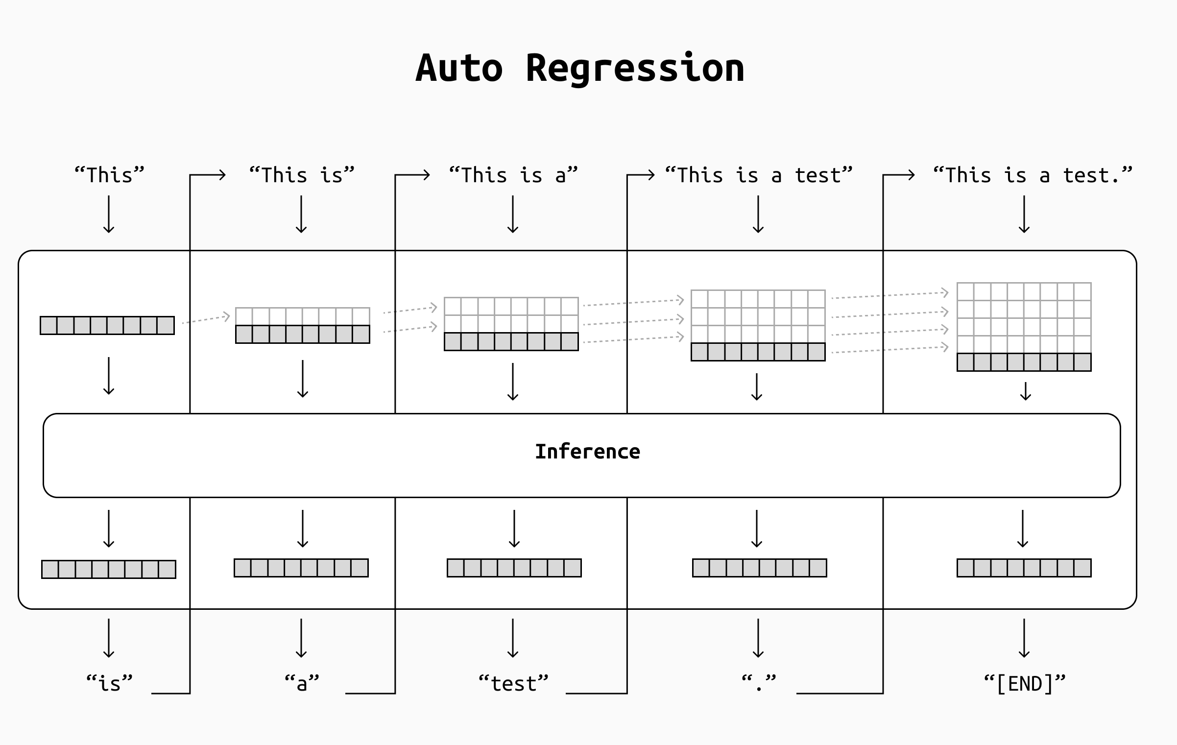
If we could somehow reuse part of the computations we did during earlier passes and only process new information as it arrives, not only the computation speed will increase dramatically, but it will stay constant during the process instead of slowing down as more tokens are generated.
This is not only true during a single request (because we won't be recomputing the whole state from the start of the message for every new token we're generating), but also across requests in the same chat (by storing the state at the end of the last assistant token) and across different chats as well (by storing the state of shared prefixes such as system prompts).
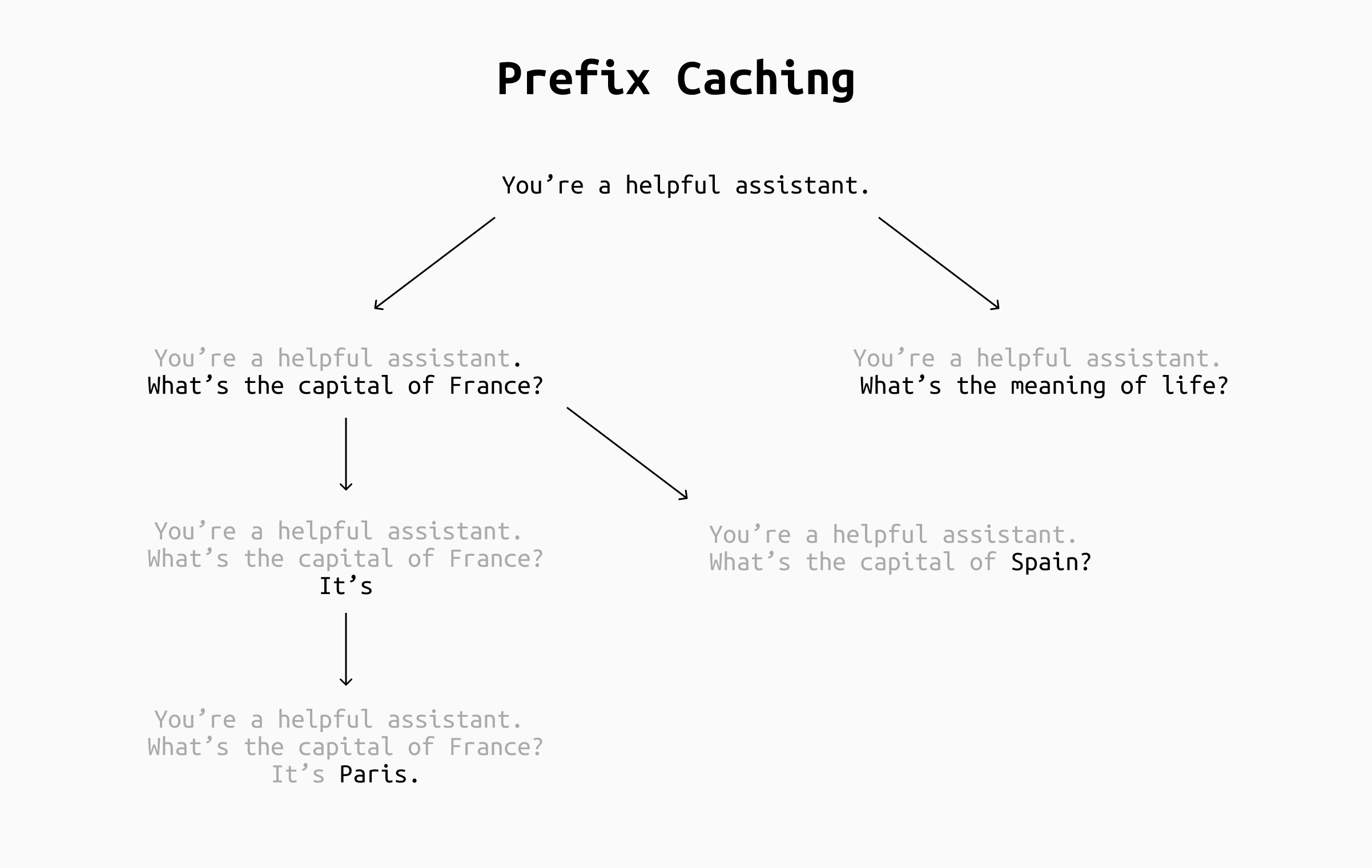
Example of prefix caching in different scenarios (gray text is caches, black is processed). By caching the system prompt, its cache can be reused with every new chat. By also caching by longest prefix, the prompts may occasionally match across chats, although it depends heavily on your applications. In any case, caching the chat as it progresses keeps the number of new tokens to process during the chat to one, making inference much faster.
But how can it be done? What exactly do we need to cache? To understand this we need to go one step deeper.
The inference process
At a high level, the inference process of a modern decoder-only Transformer such as a GPT works as follows.
- Tokenization: The chat history is broken down into tokens by a tokenizer. This is a fast, deterministic process that transforms a single string into a list of sub-word fragments (the tokens) plus a bunch of signalling tokens (to delimit messages, to signal the end of the message, to distinguish different types of input or output tokens such as thinking tokens, function calls, system prompts, etc)
- Embedding: the tokenized text passes through an embedding step, where each token is translated into an embedding (a 1-dimensional vector) using a lookup table. At this point, our input text has become a matrix of values with as many rows as tokens, and a fixed number of columns that depends on the LLM.
- Decoding: this matrix is passed through a series of 12 identical decoding steps. Each of these blocks outputs a matrix of the same shape and size of the original one, but with updated contents. These steps are "reading" the prompt and accumulating information to select the next best token to generate.that is passed as input to the next step
- Output: After the last decoding step, a final linear output layer projects the matrix into an output vector. Its values are multiplied by the lookup table we used during the embedding step: this way we obtain a list of values that represents the probability of each token to be the "correct" next token.
- Sampling: From this list, one of the top-k best tokens is selected as the next token, gets added to the chat history, and the loop restarts.
- End token: the decoding stops when the LLM picks an END token or some other condition is met (for example, max output length).
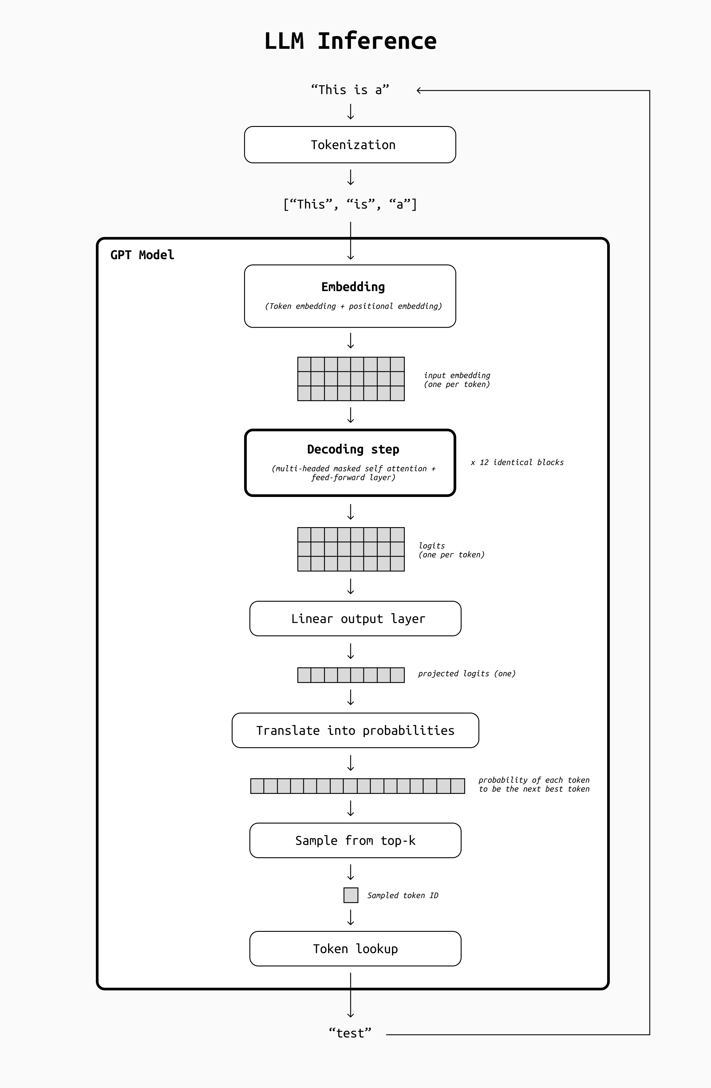
Simplified representation of the inference steps needed for an LLM to generate each output token. The most complex by far is the decoding step, which we are going to analyze in more detail.
As you can see from this breakdown, the LLM computes its internal representation of the chat history through its decoding steps, and recomputes such representation for all tokens every time we want to generate a new one. So let's zoom in even more and check what's going on inside these decoding steps.
The decoding step
LLMs may have a variable number of decoding steps (although it's often 12), but they are all identical, except for the weights they contain. This means that we can look into one and then keep in mind that the same identical process is repeated several times.
Each decoding step contains two parts:
- a multi-headed, masked self-attention layer
- a feed-forward layer
The first layer, the multi headed masked self attention, sound quite complicated. To make things easier, let's break it down into smaller concepts.
Attention is the foundation of the Transformers' incredible text understanding skills and can be roughly summarized as a technique that shows the model which tokens are the most relevant to the token we're processing right now.
Self attention means that the tokens we're looking at belong to the same sentence we're processing (which is not the case, for example, during translation tasks where we have a source sentence and a translation).
Masked self attention means that we're only looking at tokens that precede the one we're processing (which is not the case, for example, in encoder models such as BERT that encode the whole sentence at once).
Multi-headed attention means that the same operation is performed several times with slightly different parameters. Each set of parameters is called an attention head.
To understand what attention does, let's take the sentence "I like apples because they're sweet". When processing the token "they", the masked self-attention layer will give a high score to "apples", because that's what "they" refers to. Keep in mind that "sweet" will not be considered while processing "they", because masked self-attention only includes tokens that precede the token in question.
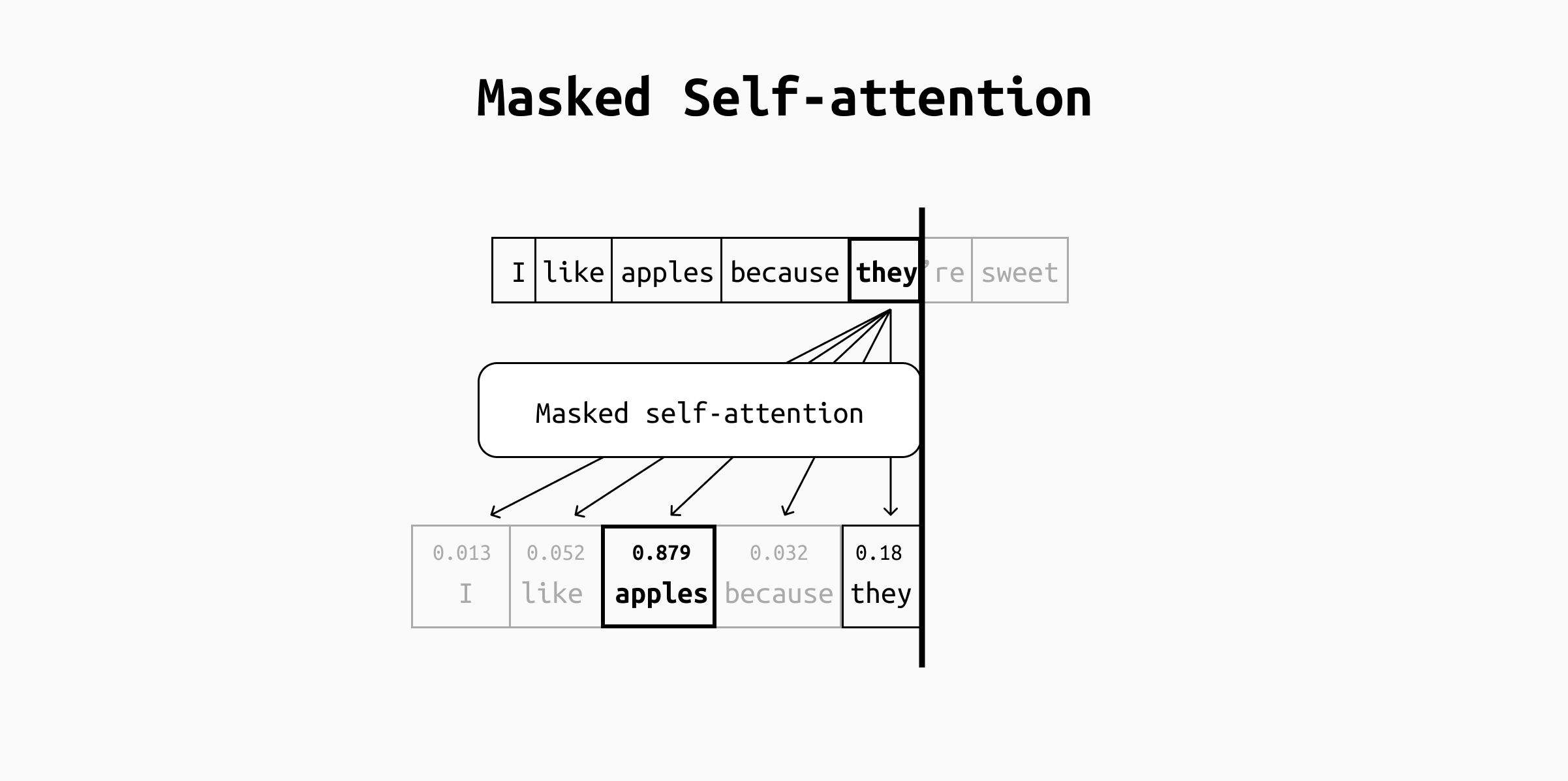
A simplified visualization of a masked self-attention head. For each token, the attention calculations will assign a score to each preceding token. The score will be higher for all preceding tokens that have something to do with the current one, highlighting semantic relationships.
The Q/K/V Matrices
Let's now look at how is this score calculated. Self-attention is implemented as a series of matrix multiplications that involves three matrices.
- Q (Query matrix): The query is a representation of the tokens we are "paying attention to" (for example, "they". In practice all tokens will be computed at the same time, so we will be dealing with a Q matrix).
- K (Key matrix): Key vectors are like labels for all the other preceding tokens in the input. They’re what we match against in our search for relevant tokens (for example "I", "like", "apples", etc ). Each token will only see the keys of tokens that precede it, so the query of "they" will not be multiplied with the key for "sweet".
- V (Value matrix): Value vectors are actual token representations. Once we’ve scored how relevant each token is, these are the values we add up to represent the token we're paying attention to. In our example, this means that the vector for "they" will be computed as a weighted average of all the previous tokens ("I", "like", "apples", "because"), but "apples" will be weighted much higher than any other, so the end result for the token "they" will be very close to the value vector for "apples".
These Q/K/V matrices are computed by multiplying the input of the decoding layer by three matrices (Wq, Wk and Wv) whose values are computed during training and constitute many of the LLM's parameters. These three matrices are addressed together as an attention head, as we mentioned earlier. Modern LLMs usually include several attention heads for each step, so you'll have several different matrices in each decoding step (and that's why they're said to use multi-headed attention).
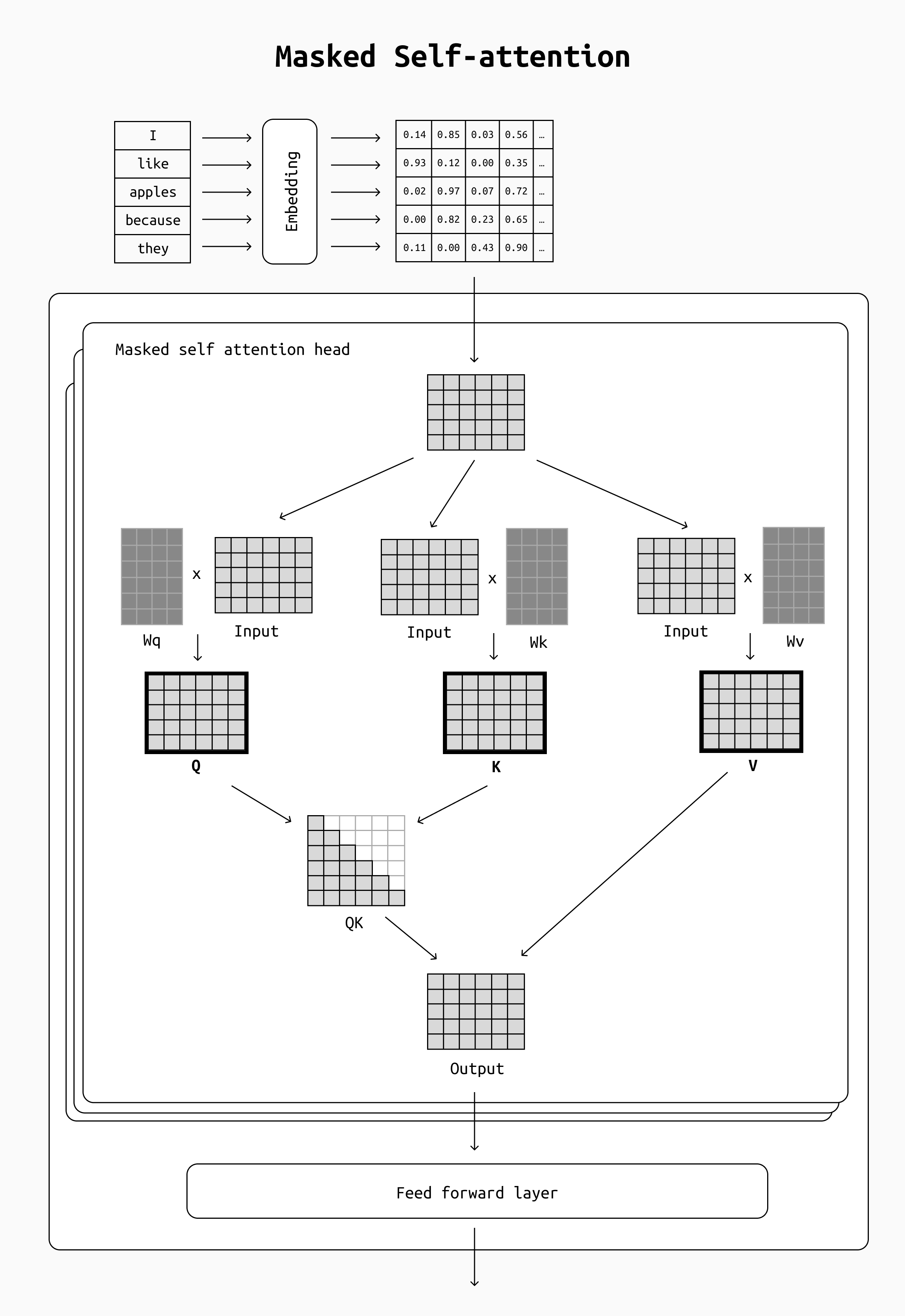
Simplified view of the Q/K/V matrices in a single self-attention head. The matrices go through a few more steps (softmax, regularization etc) which are not depicted here.
This process of computing the output vector for each token is called scaled dot-product attention and, as we mentioned earlier, happens in every attention head of every decoding step. In summary, keys (K) and values (V) are the transformed representations of each preceding token that are used to compute attention, and they enable each token to gather information from the rest of the sequence by matching queries to keys and aggregating values.
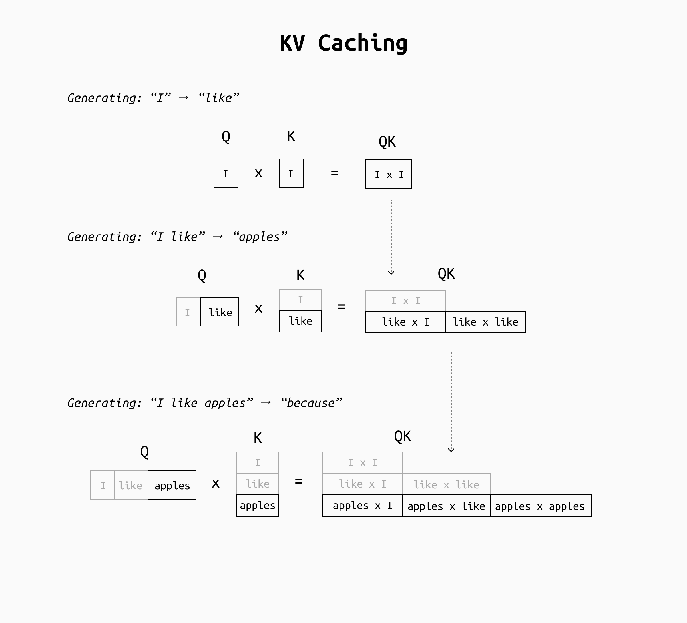
Let's pay close attention to these computations. We know that LLMs generate output one token at a time. This means that the LLM will recompute the K-V values for the tokens of the prompt over and over again for each new output token it generates. If you have already generated, say, 100 tokens of output, producing the 101st token requires recomputing a forward pass over all 100 tokens. A naive implementation would repeatedly recalculate a lot of the same intermediate results for the older tokens at every step of generation.
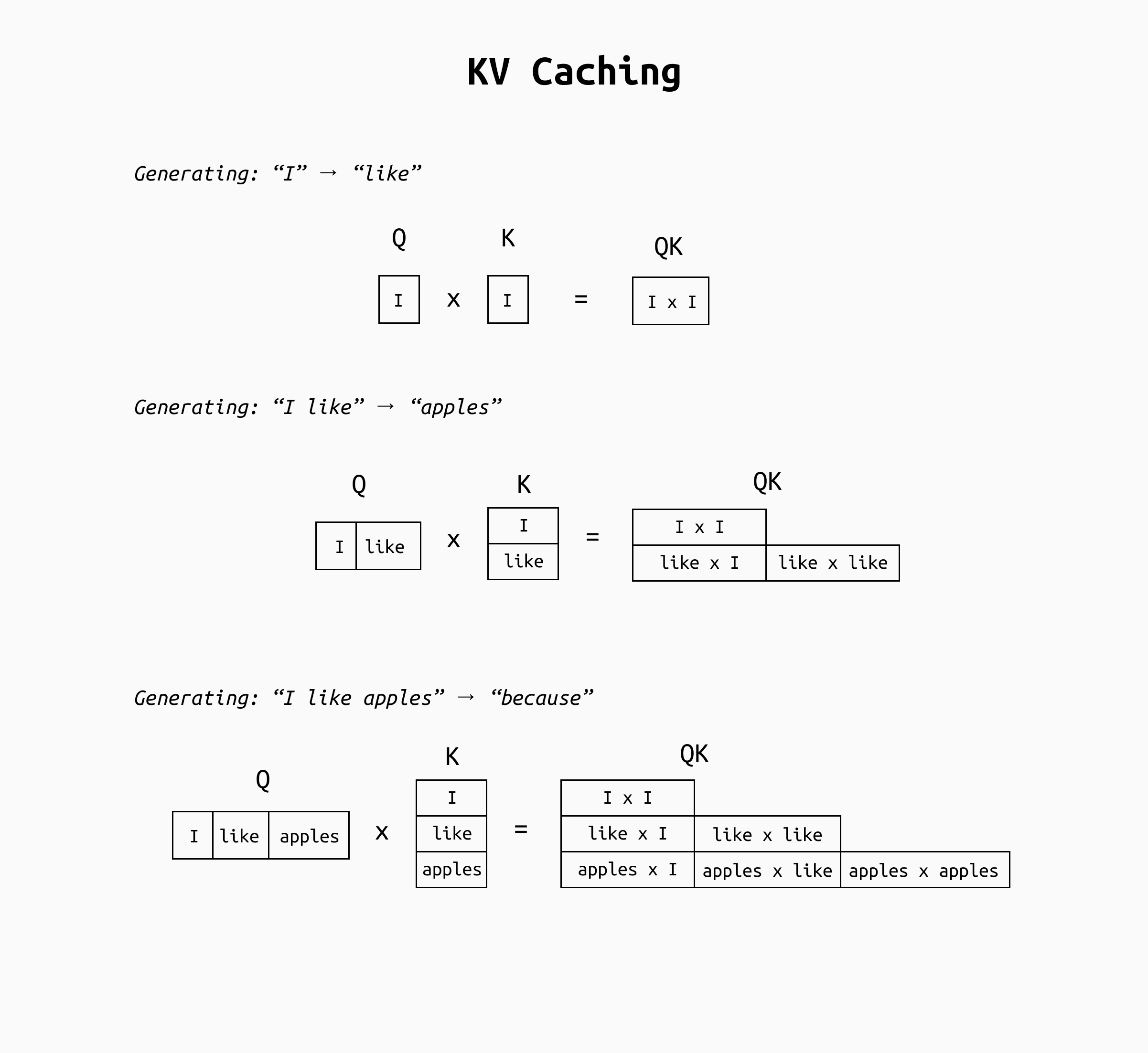
Detail of the Q/K multiplication. As you can see, the content of the QK matrix is essentially the same at all steps, except for the last row. This means that as soon as we accumulate a few input tokens, most of the QK matrix will be nearly identical every time. Something very similar happens for the final QKV matrix.
By the third generation step (three tokens in context), the model computes six attention scores (a 3×3 / 2 matrix); many of these correspond to interactions that were already computed in earlier steps. For example, the attention of token "I" with itself was computed in the first step, yet the naive approach computes it again when processing the sequence "I like" and "I like apples" and so on. In fact, by the time the sentence is complete, the majority of the query-key pairs being calculated are repeats of prior computations. This redundancy makes inference much slower as the sequence length grows: the model wastes time recalculating attention contributions for tokens that haven’t changed.
Clearly we want to avoid recomputing things like the key and value vectors for past tokens at every step. That’s exactly what KV caching achieves.
The KV Cache
KV caching is an optimization that saves the key and value tensors from previous tokens so that the model doesn’t need to recompute them for each new token. The idea is straightforward: as the model generates tokens one by one, we store the keys and values produced at each layer for each token in a cache (which is just a reserved chunk of memory, typically in GPU RAM for speed). When the model is about to generate the next token, instead of recomputing all keys and values from scratch for the entire sequence, it retrieves the already-computed keys and values for the past tokens from this cache, and only computes the new token’s keys and values.
Computing the QK matrix by reusing the results of earlier passes makes the number of calculations needed at each step nearly linear, speeding up inference several times and preventing slowdowns related to the input size.
In essence, with KV caching the transformer's attention in each layer will take the new token’s query and concatenate it with the cached keys of prior tokens, then do the same for values, and move on immediately. The result is that each generation step’s workload is greatly reduced: the model focuses on what’s new instead of re-hashing the entire context every time.
Implementation
Modern libraries implement KV caching under the hood by carrying a “past key values” or similar object through successive generation calls. For example, the Hugging Face Transformers library’s generate function uses a use_cache flag that is True by default, meaning it will automatically store and reuse past keys/values between decoding steps. Conceptually, you can imagine that after the first forward pass on the prompt, the model keeps all the K and V tensors. When generating the next token, it feeds only the new token through each layer along with the cached K and V from previous tokens, to compute the next output efficiently.
In summary, KV caching transforms the workload of each generation step. Without caching, each step repeats the full attention computation over the entire context. With caching, each step adds only the computations for the new token and the necessary interactions with prior tokens. This makes the per-step cost roughly constant. The longer the generation goes on, the more time is saved relative to the naive approach. KV caching is thus a time-memory trade-off: we trade some memory to store the cache in order to save a lot of compute time on each step.
Limitations
It’s important to note that KV caching only applies in auto-regressive decoder models (where the output is generated sequentially). Models like BERT that process entire sequences in one go (and are not generative) do not use KV caching, since they don’t generate token-by-token or reuse past internal states. But for any generative LLM built on a decoder-only Transformer architecture, KV caching is a standard technique to speed up inference.
It's worth noting that the KV cache needs to be managed just like every other type of cache. We're going to analyze some ways to handle this cache effectively in another post.
Conclusion
The takeaway is clear: always leverage KV caching for autoregressive LLM inference (and practically all libraries do this for you) unless you have a very specific reason not to. It will make your LLM deployments run faster and more efficiently.
KV caching exemplifies how understanding the internals of transformer models can lead to substantial engineering improvements. By recognizing that keys and values of the attention mechanism can be reused across time steps, we unlock a simple yet powerful optimization. This ensures that even as our LLMs get larger and our prompts get longer, we can keep inference running quickly, delivering the snappy responses users expect from AI-driven applications.
Learn more
Here are some useful resources I used to write this post:
- The Illustrated Transformer by Jay Alammar
- The illustrated GPT-2 by Jay Alammar
- Latency optimization tips by OpenAI
- KV Caching explained by João Lages
- KV Caching by Neptune.ai
- Build a Large Language Model (from scratch) by Sebastian Raschka