Making sense of KV Cache optimizations, Ep. 2: Token-level
Let's make sense of the zoo of token-level techniques that exist out there.
In the previous post we've seen what the KV cache is and what types of KV cache management optimizations exist according to a recent survey. In this post we are going to focus on token-level KV cache optimizations.
What is a token-level optimization?
The survey defined token-level optimizations every technique that focuses exclusively on improving the KV cache management based on the characteristics and patterns of the KV pairs, without considering enhancements from model architecture improvements or system parallelization techniques.
Here is an overview of the types of optimizations that exist today.
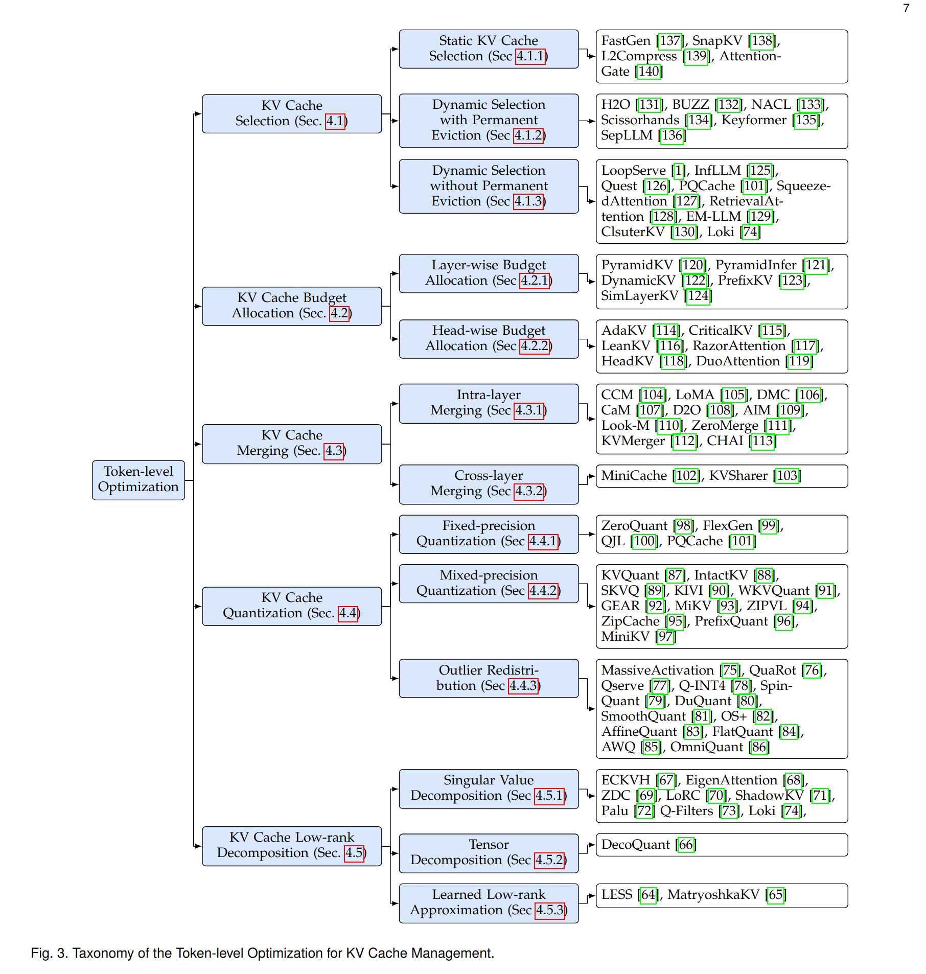
Let's see what's the idea behind each of these categories. We won't go into the details of the implementations of each: to learn more about a specific approach follow the links to the relevant sections of the survey, where you can find summaries and references.
KV Cache Selection
One key characteristic of the attention matrix is sparsity: most of its values are very close to zero, and just a few cells have meaningful values. Instead of retrieving a full matrix of attention values every time (and retrieve a ton of close-to-zero, nearly useless values), KV Cache selection techniques identify the most relevant token pair and cache those only, reducing memory utilization and inference latency.
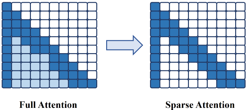
A simplified view of a cache selection strategy. In this case, the KV cache tends to have its highest values clustered near the diagonal (because most tokens refer to other tokens that are relatively close), so most of the lower-left side of the matrix can be safely assumed to be zero. That reduces drastically the number of values to store.
The researches identified two main cache selection strategies:
- Static KV cache selection. In this family of optimizations, the KV cache compression only happens during the first decoding pass (when most of the prompt is loaded in the LLM state, also called prefill phase) and remain fixed during all subsequent decoding steps, with no more compressions as the inference proceeds.
- Dynamic KV cache selection, which continuously updates and compresses the KV cache during all inference passes, enabling adaptive cache management. In dynamic KV cache selection, KV cache tokens that are not selected may be either permanently evicted or offloaded to hierarchical caching devices such as CPU memory. While more efficient in terms of memory usage, real-time KV cache selection during decoding may incur substantial computational overhead, which is usually the focus of any new technique developed in this space.
The tradeoff between static and dynamic KV cache selection is again one of latency versus efficiency, or time vs space usage. Static KV cache selection is faster and slightly less efficient; dynamic KV cache compression is more efficient in terms of memory usage but has a sensible impact on inference speed and may cause issues due to excessive compression, throwing away or putting in cold caches token pairs that are actually relevant. A clear consensus about where the sweet spot lays hasn't been found yet, and it's mostly still open to investigation.
For a more detailed description of each technique, check out the survey.
KV Cache Budget Allocation
LLMs are hierarchical, with several layers within layers of computations. Each of these layers is identical in structure, but during training the weights that they learn make some of these layers more important than others and more impactful on the output's quality.
This means that not all of these steps should be compressed equally. If we could identify which layers are more impactful we could reduce the compression of the KV cache for these layers and increase it for the others. In this way the effects of compression on the output quality would be minimized.
Budget allocation strategies tend either of these granularity levels:
- Layer-wise budget allocation, which assigns different compression ratios across the model's decoding layers
- Head-wise budget allocation, which enables precise memory distribution across individual attention heads within each layer.
Despite recent advances and growing attention in this subset of techniques, there are still big question marks about how to distribute this computing budget in an effective way. For instance, a notable discrepancy exists between pyramid-shaped allocation strategies that advocate larger budgets for lower layers, and retrieval head-based studies, which demonstrate that lower layers rarely exhibit retrieval head characteristics and thus require minimal cache resources. On top of this, there is a lack of comprehensive experimental comparisons, such as the compatibility and performance benefits of head-wise budget allocation strategies with state-of-the-art frameworks like vLLM.
For a more detailed description of each technique, check out the survey.
KV Cache Merging
The idea behind KV cache merging is to compress or consolidate separate KV caches into a single one without significantly degrading model accuracy. This stems from the observation that the various layers and attention heads often shows redundant patterns that could be merged into one single representation to improve compression.
Just like with the budget allocation techniques, KV cache merging strategies can be categorized into two primary approaches:
- Intra-layer merging, which focuses on consolidating KV caches within individual layers to reduce memory usage per layer
- Cross-layer merging, which targets redundancy across layers to eliminate unnecessary duplication.
In general, KV cache merging can be very effective at optimizing memory utilization in LLMs by consolidating KV caches while maintaining high model accuracy, and it's an active research direction that could provide more results in the near future by addressing narrower niches such as fine-tuning and adaptive merging strategies.
For a more detailed description of each technique, check out the survey.
KV Cache Quantization
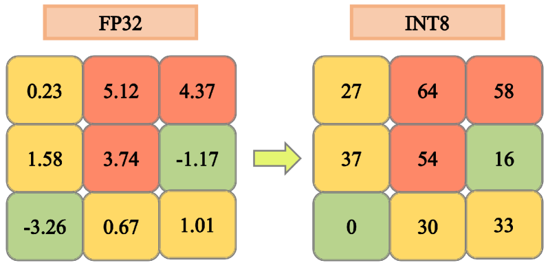
A simplified example of cache quantization. Reducing the precision of the values from float to int8 can drastically reduce the memory needs of the cache and accelerate inference.
Quantization techniques aim to convert full-precision values into integers, reducing computational and storage requirements. Quantization has also been used on other aspects of the LLM inference and training processes, such as with model parameters and data features quantization. KV cache quantization works in a similar way: by reducing the precision of numerical representations (e.g., from FP32 to INT8 or INT4) we can drastically compress the size of the KV cache and achieve up to 4x or more memory savings with respect to the full-precision floating point representation.
One of the main challenges of KV cache quantization is the presence of outliers, especially when quantizing to a very low-bit representation. These extreme values, when reduced to a smaller magnitude, can lead to a substantial performance degradation.
Depending on how they address this issue, quantization techniques can be grouped into three types:
- Fixed-precision quantization, where all Keys and Values are quantized to the same bit-width.
- Mixed-precision quantization, which assigns higher precision to critical parts of the cache while using lower precision for less important components.
- Outlier redistribution, which redistributes or smooths the outliers in Keys and Values to improve quantization quality. Some approaches to outliers redistribution include redistributing the outliers into newly appended virtual tokens or applying equivalent transformation functions to smooth the keys and values for improved quantization accuracy.
For a more detailed description of each technique, check out the survey.
KV Cache Low-rank Decomposition
Existing studies have demonstrated that the majority of information within KV caches can be captured by a small subset of their singular elements or sub-matrices with a smaller dimension, called low-rank components. Decomposing the matrix into low-rank components can effectively reduce memory requirements while preserving output quality by "picking out" the components of the KV matrix that matter the most and throwing out the rest.
Currently there are three main ways to perform low-rank decomposition of the cached KV matrix:
- Singular Value Decomposition (SVD): retains the most critical singular values.
- Tensor Decomposition: factorizes KV matrices into smaller matrices/tensors.
- Learned Low-rank Approximation: adaptive mechanisms to optimize compression based on learned low-rank representations.
Current methods primarily rely on fixed low-rank approximations applied uniformly across all layers or tokens, but future advancements could focus on dynamic rank adjustment, where the rank is tailored based on token importance, sequence length, or layer-specific properties.
For a more detailed description of each technique, check out the survey.
Conclusion
This was just a brief overview of the various techniques that have been tested to compress the KV cache, but the exploration of the space between highest accuracy, fastest inference and strongest compression is far from complete. Most of these techniques optimize for just one or two of these properties, with no clear winner that beats them all. Expect a lot more experimentation in this field in the months and years to come.
On the other hand, these are only compression techniques that apply at the token-level, without any support from the model architecture. For model-level approaches to the problem, check out the next post, where we continue exploring the survey to see how the basic architecture of the Transformer's decoding layer can be optimized to reduce the amount of values to cache in the first place.
In the next post we're going to address model-level optimizations. Stay tuned!